Stable Fluids implemented in Python/NumPy

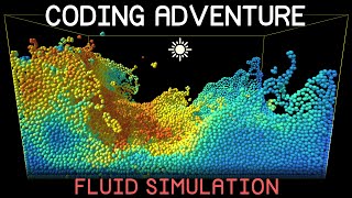
In his 1999 SIGGRAPH Paper Jos Stam introduced a famous algorithm that is still ubiquitous in Computer Graphics and Video Game Physics. It solves the Navier-Stokes equations unconditionally stable and simulates fluid dynamics. Here is the code: https://github.com/Ceyron/machine-learning-and-simulation/blob/main/english/simulation_scripts/stable_fluids_python_simple.py Unconditionally stable means that the time steps can be chosen arbitrarily large, and the kinematic viscosity can also be selected freely. This is extremely advantageous for computer graphics applications. Surely, this algorithm is unable to compete with state-of-the-art CFD codes in terms of accuracy and modelling capabilities. However, I think it is beautiful and encourages one to dig deeper. You can find Jos' original paper here: https://d2f99xq7vri1nk.cloudfront.net/legacy_app_files/pdf/ns.pdf His modified solver which is suitable to run in real-time is described here: http://graphics.cs.cmu.edu/nsp/course/15-464/Fall09/papers/StamFluidforGames.pdf ------- 📝 : Check out the GitHub Repository of the channel, where I upload all the handwritten notes and source-code files (contributions are very welcome): https://github.com/Ceyron/machine-learning-and-simulation 📢 : Follow me on LinkedIn or Twitter for updates on the channel and other cool Machine Learning & Simulation stuff: https://www.linkedin.com/in/felix-koehler and https://twitter.com/felix_m_koehler 💸 : If you want to support my work on the channel, you can become a Patreon here: https://www.patreon.com/MLsim ------- Timestamps: 00:00 Introduction 00:23 About Stable Fluids 00:59 Problem Scenario 01:14 Upwards Forcing 01:31 Algorithm in Detail 04:06 Note on Boundary Conditions 04:17 Imports 05:11 Defining Simulation Parameters (=Constants) 05:53 Some Boilerplate 06:07 Creating a mesh 09:24 Forcing Function Definition 11:39 Vectorizing the Forcing Function 12:33 Time Loop + Initial condition 13:09 Step 1: Apply forces 13:50 Step 2: Nonlinear Convection (Self-Advection) 17:04 Step 3: Diffuse 17:19 Laplace Operator 18:58 Implicit Diffusion Operator 20:46 Step 3: Diffuse (cont.) 22:30 Step 4.1: Compute Pressure 23:00 Divergence + Partial Derivatives 26:00 Poisson Operator 26:54 Step 4.1: Compute Pressure (cont.) 27:53 Step 4.2: Pressure Correction 28:07 Gradient Operator 29:31 Step 4.2: Pressure Correction (cont.) 30:04 Advance in time 30:22 Initial visualization 31:43 First run + debugging 32:47 Curl Operator 34:00 Visualizing the Curl 36:15 Discussing the Plot 36:51 Playing with the Viscosity 37:20 Instability 37:56 Outro